| |
SOLAR RADIATION AND CLIMATE
OF THE EARTH |
|
V.M.
Fedorov, A.A. Kostin Introduction Solar radiation arriving to the Earth alters both in time and space. Variation of arriving solar radiation is determined by two basic reasons, which have different physical nature. First, solar radiation variations are determined by the Sun physical activity shift (Willson, 1982; Frohlich, 1989; Frohlich et al., 1998; Makarova et al., 1991; Foukal et al., 2006; Willson, Mordvinov, 2003; http://www.sidc.be; http://www.pmodwrc.ch). The said variations are not considered in our calculations. Second, variations of solar radiation arriving to the Earth are determined celestially, by mechanical processes. These variations of solar stream, until the present day, have been basically studied in geological scale of time which is known to be rather sustained. Calculations of solar radiation, however, do not cover such astronomical elements, exposed to secular perturbations, as longitude of perihelion, ellipticity, Earth's axis inclination, which have long (tens of thousands years) periods of variations. Periodical perturbations of the Earth's orbit elements in this case are not considered (Milankovich, 1939; Brouwer, Van Woerkom, 1950; Sharaf, Budnikova, 1969; Vulis, Monin, 1979; Berger, Loutre, 1991, Monin, Shishkov, 2000). Calculations within the range of the Earth's orbit elements periodical perturbations and solar radiation variations connected with them, were started in A. I. Voyeikov Main Geophysical Observatory (Borisenkov, 1983). However, this research did not result in any further development. Though, calculations of solar radiation arriving to the outer fringe are believed to be of importance, since the acquired values are an initial basis for the Earth radiation balance and its specific geospheres. Opposed to the approach of M. Milankovich (Milankovich, 1939) and his successors (Brouwer, Van Woerkom, 1950; Sharaf, Budnikova, 1969; Vulis, Monin, 1979; Berger, Loutre, 1991), who considered long-term intervals of time, we made a point of a more detailed calculation for solar radiation arriving over a shorter time interval. In which case, we took into account the Earth’s orbit elements and Earth axis inclinations periodical perturbations. Basic ideas of our approach are: distance from the Earth to the Sun and Earth axis orientation are taken from NASA’s accurate model DE-406 (http://ssd.jpl.nasa.gov), Earth ellipsoid is divided into latitudinal bands, and each tropical year—into segments, and each pair (band, segment) is associated with an integral (J) of insolation (W/m2) to a band from end to end of a segment. By dividing the integral by a band square we obtain specific energy (J/m2), collected by a band within a segment. By multiplying the integral by ratio of a band fragment length to the band length we obtain assessed value of energy (J), collected by this fragment within the segment. To calculate the said values, a number of theoretical simplications was introduced. Basic simplications: solar activity is considered constant, irradiation—coming from the centre of the Sun, Earth atmosphere influence is ignored. All theoretical simplications are stated in section 1. Pure formulae for calculations are given in section 2. Tried technology of rough calculations and their typical tolerance are discussed in section 3. Tendencies of arriving solar radiation variation are discussed in section 4.
1. The selected approach towards description of arriving solar radiation Considered period of time is from 3000 BC to 2999 AD. The Earth’s surface approximates ellipsoid, hereinafter referred to as MRS80, swaying against geoid, with major semiaxes lengths of p1=p2=A=6378137 m and minor semiaxis length of p3=B=6356752 m. Minor semiaxis at each moment lies in the Earth’s axis, and ellipsoid centre—in geocenter. Semiaxes lengths with rounding to one meter correspond to parameters of overall Earth ellipsoid GRS80, which is fixed relative to geoid1. Swaying ellipsoid MRS80 is provided with imaginary scale of parallels and meridians, system of normals and geodetic coordinates, whereby vertical lines, horizontal planes and latitudinal zones of Earth are determined. These lines, planes and zones together with ellipsoid slightly sway against the geoid. Swayings are connected with the Earth’s axis inclination from its midposition within the Earth body. Inclinations have been registered from the end of the 19th century in terms of geographic poles movement2. Swaying ellipsoid has been chosen instead of a fixed one for two reasons: first: to avoid adding complexity to calculations, and because of the lack of a sound swaying model, which would embrace the whole time span examined. In the absence of obstacles for rays, solar radiation which achieves a given point of the Earth surface, in general, will be resolved on vertical (normally against the surface) and horizontal (horizontal tangent against the surface) constituents. Vertical constituent hereinafter will be referred to as falling vertical radiation (FVR). We consider a model of solar radiation and its imaginary measurement on the Earth’s surface according to which: 1) isotropic radiation comes to the Earth from the center of the Sun3, 2) eclipses are ignored, 3) radiation power density at a distance of 1 A.U. from the center of the Sun at each moment equals to u0=1367 W/m2, where 1 A.U. =r0=149597870691 m, 4) dissipating effect of the atmosphere is ignored, 5) the Earth’s surface is substituted with swaying ellipsoid MRS80. Swaying ellipsoid is split into FVR integrals are calculated – energy
(in Joules), arriving to the Earth via each of the bands in each of
the Tropical years were chosen instead of
calendar years to avoid the four-year calendar rhythmics. Number of
a tropical year aligns with the number of the calendar year within which
it starts. Tropical year stands for projective tropical year tracked
by movement of the Sun projection against ecliptic. If To take account of day elongation due to gradual slow-down of the Earth rotation we differentiate the calendar time scale within which a single day corresponds to a massive of 86400 calendar seconds, and scale of uniformly running time, according to which daily intervals are measured in true seconds and are not equal to each other. Solar radiation integrals are calculated according to scale of uniformly running time. Imaginary clock keeping account of uniformly running time is situated in the center of the Earth. An event on a small area of the Earth (“a dose of solar radiation arrived”) is related to the axle of uniformly running time in the following way. We assume a moment of a corresponding dose bundle imaginary start from the center of the Sun. A dose directed towards the center of the Earth is deposited from this bundle. A moment of imaginary arrival of this dose to the Earth’s center is calculated (assuming absence of obstacles on its way). This arrival moment is selected as the one to which the said event shall be related to. Small (20-40ms) delays (various in various areas of a band) may emerge for this way of relation. Although, from the point of view of large scale Earth processes such systematic delays of relation are omissible. They are equivalent to small (about 30ms) displacements of tropical years segments boundaries. A variant with delays has been chosen for the reason that their exclusion could result in excessive complication of calculations.
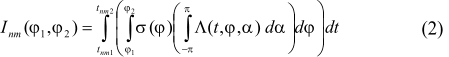
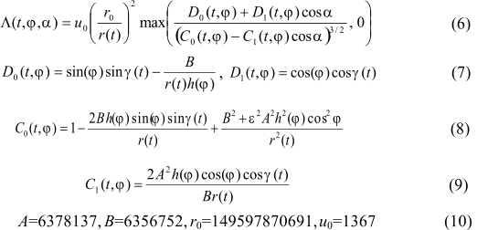
2. Pure Formulae for Calculations According to the chosen model of
solar radiation and its measurement, calculation of FVR integrals (in
Joules) leans upon calculation of vertical insolation Elementary fragment of a tropical year
may be obtained via its splitting into 360 parts. FVR energy, arriving
to the Earth via a band of enclosing surface, limited by latitudes
Let us assume that
where
Let
Before integrating by formula (2), it
would be useful to ask yourself: if If One of the properties of vertical insolation
is evenness by
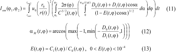
3. Approximate calculation and
their errors in case of 3.1. Plan of calculations Calculations by formulae (1), (3)-(13) cannot be made with absolute accuracy. Inaccuracies are peculiar for initial data, procedures of interpolation and search of equation roots during processing of initial data and integration procedures. For a variant when The first stage is a work marking of the
used time scales, addressing to the HORIZONS NASA internet-service (http://ssd.jpl.nasa.gov/?horizons_doc#specific_quantities;
Giorgini et al., 1996) The second stage is calculation of displacements of tropic years elementary fragments starts and ends in relation to starts of days GMT (for this, search of equations roots with participation of ecliptic longitude) and, at this basis, gathering of secondary initial data, associated with starts, ends and intermediate moments of elementary fragments of tropic years (for this there is interpolation of primary data). Secondary initial data are: distance Earth-Sun (m), declination of the Sun (radians), and durations of fragments (с) at the scale of uniformly flowing time. The third stage is calculation of FVR integrals by means of secondary initial data (for this there is calculation of auxiliary variables and their substitution into integration procedures).
3.2. Three time scales and their work marking There are three scales used: CT (Coordinate
Time – coordinate, the same as uniformly flowing time), UT1 (Universal
Time Without Correction – continuous worldwide time) and UT2=UTC (Universal
Time With Correction – discontinuous worldwide time). Scale UT2 results
from scale UT1 by episodical (once in several years) movements by Measurement unit of scale СТ is a true
second. At CT scale there are two markings: tropical and calendar. Tropical
marking consists of main moments
Tropic marking spreads from the first
fragment of tropic year 3000BC till the last fragment of tropic year
2999AD. True duration
Calendar marking
Further we use functions
Their sense:
Sequence
3.3. Retrieval of primary initial data Primary initial data is a block of values
of type Primary initial data was retrieved by us from ephemerides NASA DE406 by means of the HORIZONS internet-service. In the inquiries made we set the following parameters (for Time Span there is an example): Ephemeris
Type = OBSERVER,
3.4. Calculation of secondary initial data by primary data Secondary initial data is a block of values
of the type
Formulae of spline-interpolation application:
where
Root of each equation of the type (32) is sought by approximation method with a roughness of 10–9 (in a day).
3.5. Calculation of FVR integrals by means of secondary initial data After pass from (2) to (11), further siplification
consists in approximate analytic integral evaluation by
and omitting, for short, arguments
During integration
Before integration by
Each summand within the integral sum by
Integral
As a result, practical evaluation of FVR integrals is performed based on secondary initial data by formulae (1), (40), (50), (41), (48), (49) with the use of (42)-(47), (35)-(39), (12)-(13), (7)-(10), (3)-(4).
3.6. Resulting roughnesses of evaluations Resulting roughness of evaluation for each FVR integral will be at most few percents from average module of its interannual variability. Relative roughness does not exceed 0.005% for FVR integrals in the vicinity of poles and 0.00005% for FVR integrals in the vicinity of equator. Subsequent to the results of evaluation for the period from 3000 BC till 2999 AD we formed a base of radiation data for arriving (in the absence of atmosphere) solar radiation to latitude zones of the Earth (5 degrees spread) with time pitch equal to 1/12 part of tropic year. Base of radiation data is set at the site “Solar radiation and climate of the Earth” (http://solar-climate.com/en\ensc\bazard.htm).
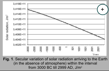
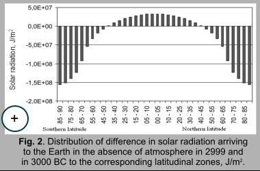
4. Secular trends in variation of arriving solar radiation Secular variability has been evaluated by difference of arriving radiation values (J/m2) during the last (2999 AD) and the first (3000 BC) year of the time interval for corresponding latitudinal zones. The results show the decrease for this period of solar radiation arriving to the outer fringe equal to 1.16E+09 J/m2 or 0.339% from average annual value of solar radiation arriving during this period (Fedorov, 2012, 2015). This trend (fig. 1) is determined by secular variations of ellipticity, Earth axis inclination and longitude of perihelion (Milankovich, 1939). Reducing stream of solar radiation, arriving to the Earth ellipsoid during tropic year in districts below 45° of latitude at each hemisphere tends to increase and above 45° – to reduce (fig. 2).
Reduction of radiation arriving to polar areas during the whole period achieves 1.58Е+08 J/m2, which is 2.8% in relation to average (for the whole interval) value of arriving radiation for latitudinal zones of 85° -90° geographic latitude. Increase within the equatorial area (exceeding polar districts by area, approximately by 2.7 times) is substantially smaller, and at equator region it equals to 3.32Е+07 J/m2 (0.25%). Consequently, one of the trends in variation of arriving solar radiation at present day is intensification of latitudinal contrast (increase of inter latitude gradient of solar radiation arriving to the outer fringe).
The decrease achieves the maximum value in this season in the Southern polar area -1.56Е+08 J/m2, which equals to 2.83% from the average annual (for the whole period) value of solar radiation arriving to this latitudinal zone. Decrease average for the 5-degree latitudinal zone during this interval (3000 BC-2999) equals to -7.55Е+07 J/m2. Total decrease of arriving radiation in the area of decrease is 1.21Е+09 J/m2. Positive values during this season are characteristic for the area of 5° -10° of the Southern latitude and for all latitudinal zones to the north from this zone. Maximum value is marked in latitudinal zone of 45 -50 N.l. is 5.42Е+07 J/m2, which equals to 2.04% of average annual value of radiation arriving to this zone in winter semester (for the Norhtern hemisphere). Increase, average for 5-degree zone, of arriving solar radiation equals to 3.14Е+07 J/m2. Increase within the area of increase is characterised by value equal to 6.29Е+08 J/m2. Overall decrease of solar radiation arriving to the Earth (to the outer fringe) during winter semester (for the Northern hemisphere) equals to -5.79 J/m2.
Maximum increase is a characteristic of the latitudinal zone of 45° -50° S.l. is 5.41Е+07 J/m2, which equals to 2.038% of average annual value of solar radiation arriving to this zone in summer semester (for the Norhtern hemisphere). Medium increase, for 5-degree latitudinal zone, in this area equals to 3.14Е+07 J/m2, and total (for the area of increase) equals to 6.29Е+08 J/m2. Decrease is marked at this time in the area of 10° -15° N.l. and to the north. Maximum decrease is a characteristic of the zone of 85° -90° N.l. and equals to -1.56Е+08 J/m2, which is 2.831% from average annual value of solar radiation arriving to this zone. Decrease, average for the 5-degree zone, equals to -7.55Е+07 J/m2, total (for the decrease area) is -1.21Е+09 J/m2. Total decrease (for the Earth) of arriving solar radiation in summer semester (for the Northern hemisphere) equals to -5.79Е+08 J/m2. Thus, increase of arriving solar radiation is marked in winter semesters (for hemispheres), and decrease is marked in summer hemispheres. Seasonal variations of solar radiation arriving to the outer fringe are hereby flattened. The marked trends (intensification of latitudinal contrast and flattening of seasonal differences) in variation of arriving solar radiation are connected with secular tendency towards decrease of the Earth axis inclination (regarding perpendicular to ecliptic plane) as a result of precession and nutation. It is known, that in case of the Earth’s axis inclination increase, radiation arrival to polar regions increases, i.e. latitudinal contrast flattening and seasonal differences intensification takes place in hemispheres. In case of gradient angle decrease radiation will grow in subequatorial regions, resulting in intensification of latitudinal contrasts, and flattening of seasonal differences (Milankovich, 1939; Monin, Shishkov, 2000)
Conclusion Based on astronomical ephemerides DE-406 evaluations of solar radiation arriving to the Earth ellipsoid have been performed (in the absence of atmosphere). Analysis of calculated values of arriving solar radiation allowed to obtain a number of interesting results: 1. Solar radiation arriving during tropic years to the outer fringe decreases. 2. Marked increase of solar radiation arriving to the Earth equatorial areas and decrease in polar areas. It means that the contemporary epoch is characterised with intensification of interlatitudinal gradient in distribution of arriving solar radiation at the outer fringe. 3. Marked decrease of arriving solar radiation in summer semesters and increase in winter ones (for hemispheres). This reflects a tendency of seasonal differences flattening in solar radiation arriving to the outer fringe. 4. Formed database of solar radiation arriving to the outer fringe (http://solar-climate.com/en\ensc\bazard.htm). These data may be used in physical and mathematical models of climate. The obtained picture of temporal and spatial changes in solar radiation arriving to the Earth may find reflection in radiation and thermal conditions of the planet. In such a way, tendency to the increase of interlatitudinal gradient of arriving solar radiation may be connected with increase of interlatitudinal temperature contrasts and intensification of interlatitudinal heat exchange, which is possibly one of the reasons for the trend of climate warming in extra tropical regions of the Earth.
|


 by
method of the 3rd degree polynom:
by
method of the 3rd degree polynom:
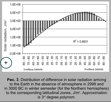 We also analysed solar radiation arriving to the outer fringe during
winter and summer semester. Secular variation was evaluated by difference
of values of arriving solar radiation (J/m2) during the last
(2999 AD) and the first (3000 BC) year of the time interval for corresponding
semesters. During winter semester (for Northern hemisphere) (fig. 3)
we registered decrease of arriving solar radiation within the latitudinal
area from 10° S.l. to 90° S.l.
We also analysed solar radiation arriving to the outer fringe during
winter and summer semester. Secular variation was evaluated by difference
of values of arriving solar radiation (J/m2) during the last
(2999 AD) and the first (3000 BC) year of the time interval for corresponding
semesters. During winter semester (for Northern hemisphere) (fig. 3)
we registered decrease of arriving solar radiation within the latitudinal
area from 10° S.l. to 90° S.l.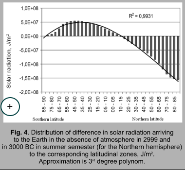 During summer semester (for the Northern hemisphere) (fig.4) increase
of arriving solar radiation is marked in the area from the zone of 5°
-10° N.l. and situated to the south.
During summer semester (for the Northern hemisphere) (fig.4) increase
of arriving solar radiation is marked in the area from the zone of 5°
-10° N.l. and situated to the south.
|
SOLAR RADIATION AND CLIMATE |
|
|||||
|
© www.solar-climate.com
|

|
|
||||||||||||||||||||||||||||||||||||||||||
|
|
|||
|
|||||||||||||


 |
 |